Of Streams and Tables in Kafka and Stream Processing, Part 1
In this article, perhaps the first in a mini-series, I want to explain the concepts of streams and tables in stream processing and, specifically, in Apache Kafka. Hopefully, you will walk away with both a better theoretical understanding but also more tangible insights and ideas that will help you solve your current or next practical use case better, faster, or both.
Update (January 2020): I have since written a 4-part series on the Confluent blog on Apache Kafka fundamentals, which goes beyond what I cover in this original article.
In the first part, I begin with an overview of events, streams, tables, and the stream-table duality to set the stage. The subsequent parts take a closer look at Kafka’s storage layer, which is the distributed "filesystem" for streams and tables, where we learn about topics and partitions. Then, I move to the processing layer on top and dive into parallel processing of streams and tables, elastic scalability, fault tolerance, and much more. The series is related to my original article below, but is both broader and deeper.
- Streams and Tables in Apache Kafka: A Primer (link is broken as of 2025)
- Streams and Tables in Apache Kafka: Topics, Partitions, and Storage Fundamentals
- Streams and Tables in Apache Kafka: Processing Fundamentals with Kafka Streams and ksqlDB
- Streams and Tables in Apache Kafka: Elasticity, Fault Tolerance, and other Advanced Concepts
- Motivation, or: Why Should I Care?
- Streams and Tables in Plain English
- Illustrated Examples
- Streams and Tables in Kafka English
- Streams and Tables in Your Daily Development Work
- A Closer Look with Kafka Streams, KSQL, and Analogies in Scala
- Tables Stand on the Shoulders of Stream Giants
- Turning the Database Inside-Out
- Wrapping Up
Motivation, or: Why Should I Care?
In my daily work I interact with many users regarding Apache Kafka and doing stream processing with Kafka through Kafka’s Streams API (aka Kafka Streams) and KSQL (the streaming SQL engine for Kafka). Some users have a stream processing or Kafka background, some have their roots in RDBMS like Oracle and MySQL, some have neither.
One common question is, “What’s the difference between streams and tables?” In this article I want to give both a short TL;DR answer but also a longer answer so that you can get a deeper understanding. Some of the explanations below will be slightly simplified because that makes them easier to understand and also easier to remember (like how Newton’s simpler but less accurate gravity model is perfectly sufficient for most daily situations, saving you from having to jump straight to Einstein’s model of relativity; well, fortunately, stream processing is never that complicated anyways).
Another common question is, “Alright, but why should I care? How does this help me in my daily work?” In short, a lot! Once you start implementing your own first use cases, you will soon realize that, in practice, most streaming use cases actually require both streams and tables. Tables, as I will explain later, represent state. Whenever you are doing any stateful processing like joins (e.g., for real-time data enrichment by joining a stream of facts with dimension tables) and aggregations (e.g., computing 5-minute averages for key business metrics in real-time), then tables enter the streaming picture. And if they don’t, then this means you are in for a lot of DIY pain. Even the infamous WordCount example, probably the first Hello World you have encountered in this space, falls into the stateful category: it is an example of stateful processing where we aggregate a stream of text lines into a continuously updated table/map of word counts. So whether you are implementing a simple streaming WordCount or something more sophisticated like fraud detection, you want an easy-to-use stream processing solution with all batteries and core data structures (hint: streams and tables) included. You certainly don’t want to build needlessly complex architectures where you must stitch together a stream(-only) processing technology with a remote datastore like Cassandra or MySQL, and probably also having to add Hadoop/HDFS to enable fault-tolerant processing (3 things are 2 too many).
Streams and Tables in Plain English
Here’s the best analogy I can think of:
- A stream in Kafka records the full history of world (or business) events from the beginning of time to today. It represents the past and the present. As we go from today to tomorrow, new events are constantly being added to the world’s history. This history is a sequence or “chain” of events, so you know which event happened before another event.
- A table in Kafka is the state of the world today. It represents the present. It is an aggregation of the history of world events, and this aggregation is changing constantly as we go from today to tomorrow.
Let’s use Chess as an example:
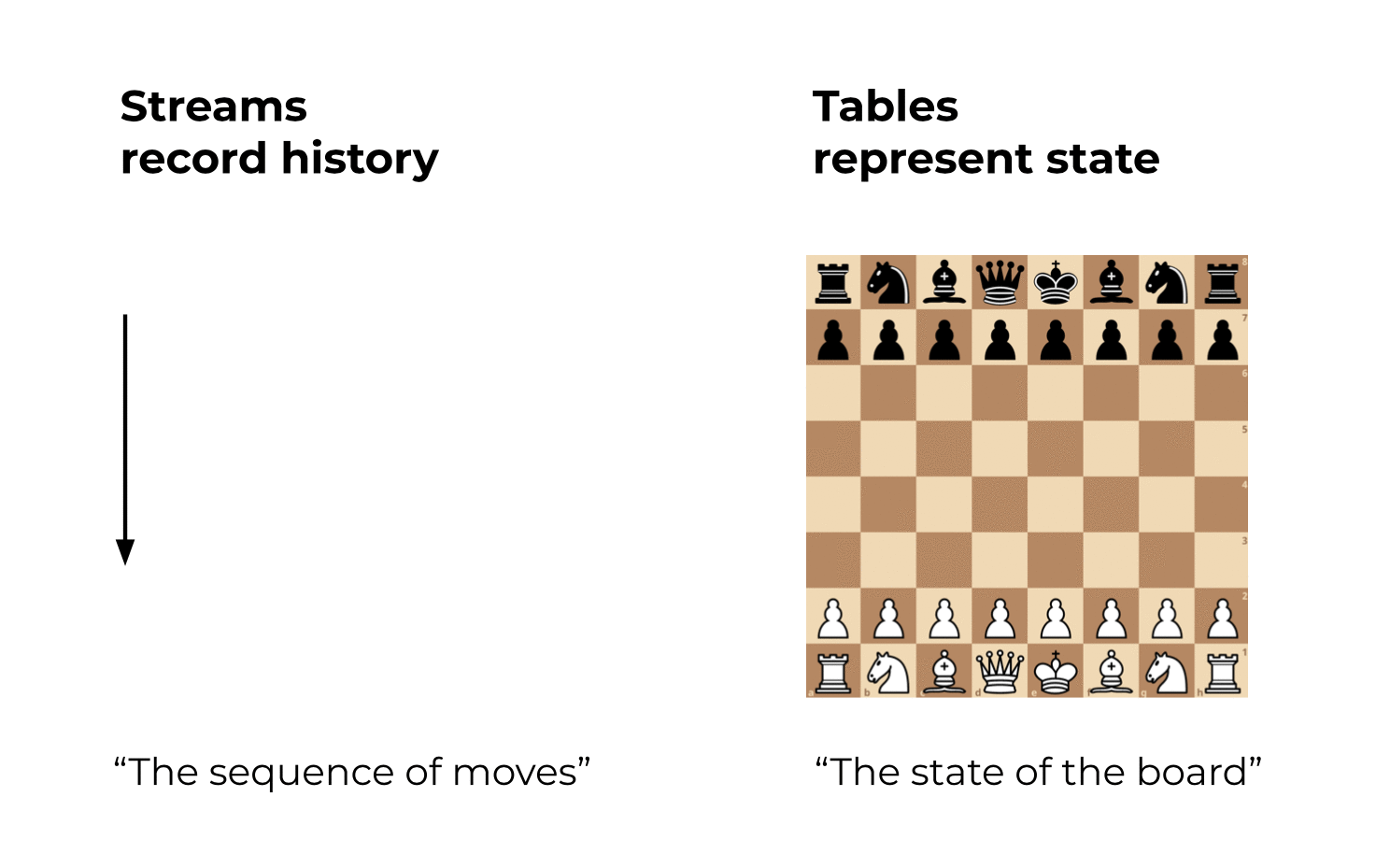
And as an appetizer for a future blog post: If you have access to the full history of world events (stream), then you can of course generally reconstruct the state of the world at any arbitrary time, i.e. the table at an arbitrary time t in the stream, where t is not restrained to be only t=now. In other words, we can create “snapshots” of the world’s state (table) for any time t, such as 2560 BC when the Great Pyramid of Giza was built, or 1993 AC when the European Union was formed.
Illustrated Examples
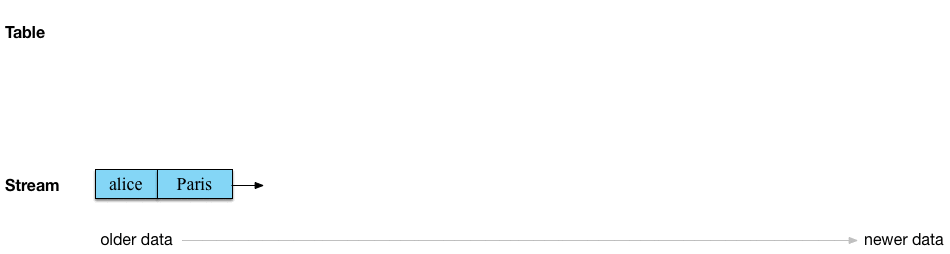
The first use case example shows a stream of user geo-location updates that is being aggregated into a table that tracks the current aka latest location for each user. As I will explain later, this also happens to be the default table semantics when you are reading a Kafka topic directly into a table.

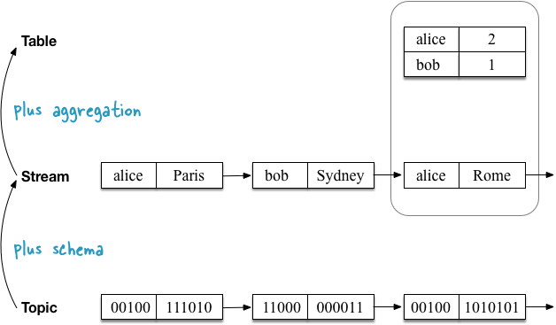
The second use case example shows the same stream of user geo-location updates, but now the stream is being aggregated into a table that tracks the number of visited locations for each user. Because the aggregation function is different (here: counting) the contents of the table are different. More precisely, the values per key are different.
Streams and Tables in Kafka English
Before we dive into details let us start with a simplified summary.
A topic in Kafka is an unbounded sequence of key-value pairs. Keys and values are raw byte arrays, i.e. <byte[], byte[]>.
A stream is a topic with a schema. Keys and values are no longer byte arrays but have specific types.
- Example: A
<byte[], byte[]>topic is read as a<User, GeoLocation>stream of geo-location updates.
A table is a, well, table in the ordinary sense of the word (I hear the happy fist pumps of those of you who are familiar with RDBMS but new to Kafka). But, seen through the lens of stream processing, a table is also an aggregated stream (you didn’t really expect we would just stop at “a table is a table”, did you?).
-
Example: A
<User, GeoLocation>stream of geo-location updates is aggregated into a<User, GeoLocation>table that tracks the latest location of each user. The aggregation step continuously UPSERTs values per key from the input stream to the table. We have seen this in the first illustrated example above. -
Example: A
<User, GeoLocation>stream is aggregated into a<User, Long>table that tracks the number of visited locations per user. The aggregation step continuously counts (and updates) the number of observed values per key in the table. We have seen this in the second illustrated example above.
Think:
Topics, streams, and tables have the following properties in Kafka:
| Concept | Partitioned | Unbounded | Ordering | Mutable | Unique key constraint | Schema |
|---|---|---|---|---|---|---|
| Topic | Yes | Yes | Yes | No | No | No (raw bytes) |
| Stream | Yes | Yes | Yes | No | No | Yes |
| Table | Yes | Yes | No | Yes | Yes | Yes |
Let’s see how topics, streams, and tables relate to Kafka’s Streams API and KSQL, and also draw analogies to programming languages (the analogies ignore, for example, that topics/streams/tables are partitioned):
| Concept | Kafka Streams | KSQL | Java | Scala | Python |
|---|---|---|---|---|---|
| Topic | - | - | List/Stream |
List/Stream[(Array[Byte], Array[Byte])] |
[] |
| Stream | KStream |
STREAM |
List/Stream |
List/Stream[(K, V)] |
[] |
| Table | KTable |
TABLE |
HashMap |
mutable.Map[K, V] |
{} |
Streams and Tables in Your Daily Development Work
Let me make a final analogy. If you are a developer, you are very likely familiar with git. In git, the commit history represents the history of the repository (aka the world), and a checkout of the repository represents the state of the repository at a particular point in time. When you do a git checkout <commit>, then git will dynamically compute the corresponding state aka checkout from the commit history; i.e., the checkout is an aggregation of the commit history. This is very similar to how Kafka computes tables dynamically from streams through aggregation.
| Concept | Git |
|---|---|
| Stream | commit history (git log) |
| Table | repo at commit (git checkout <commit>) |
So much for a first overview. Now we can take a closer look.
A Closer Look with Kafka Streams, KSQL, and Analogies in Scala
I’ll start each of the following sections with a Scala analogy (think: stream processing on a single machine) and the Scala REPL so that you can copy-paste and play around yourself, then I’ll explain how to do the same in Kafka Streams and KSQL (elastic, scalable, fault-tolerant stream processing on distributed machines). As I mentioned in the beginning, I slightly simplify the explanations below. For example, I will not cover the impact of partitioning in Kafka.
map()) are being chained together, what these operations represent (e.g. reduceLeft() represents an aggregation), and how the stream "chain" compares to the table "chain".
Topics
A topic in Kafka consists of key-value messages. The topic is agnostic to the serialization format or “type” of its messages: it treats message keys and message values universally as byte arrays aka byte[]. In other words, at this point we have no idea yet what’s in the data.
Kafka Streams and KSQL don’t have a concept of “a topic”. They only know about streams and tables. So I only show the Scala analogy for a topic here.
// Scala analogy
scala> val topic: Seq[(Array[Byte], Array[Byte])] = Seq((Array(97, 108, 105, 99, 101),Array(80, 97, 114, 105, 115)), (Array(98, 111, 98),Array(83, 121, 100, 110, 101, 121)), (Array(97, 108, 105, 99, 101),Array(82, 111, 109, 101)), (Array(98, 111, 98),Array(76, 105, 109, 97)), (Array(97, 108, 105, 99, 101),Array(66, 101, 114, 108, 105, 110)))
Streams
We now read the topic into a stream by adding schema information (schema-on-read). In other words, we are turning the raw, untyped topic into a “typed topic” aka stream.
In Scala this is achieved by the map() operation below. In this example, we end up with a stream of <String, String> pairs. Notice how we can now see what’s in the data.
// Scala analogy
scala> val stream = topic
                  |  .map { case (k: Array[Byte], v: Array[Byte]) => new String(k) -> new String(v) }

// => stream: Seq[(String, String)] =
//      List((alice,Paris), (bob,Sydney), (alice,Rome), (bob,Lima), (alice,Berlin))
In Kafka Streams you read a topic into a KStream via StreamsBuilder#stream(). Here, you must define the desired schema via the Consumed.with() parameter for reading the topic’s data:
StreamsBuilder builder = new StreamsBuilder();
KStream<String, String> stream =
  builder.stream("input-topic", Consumed.with(Serdes.String(), Serdes.String()));
In KSQL you would do something like the following to read a topic as a STREAM. Here, you must define the desired schema by defining column names and types for reading the topic’s data:
CREATE STREAM myStream (username VARCHAR, location VARCHAR)
  WITH (KAFKA_TOPIC='input-topic', VALUE_FORMAT='...')
Tables
We now read the same topic into a table. First, we need to add schema information (schema-on-read). Second, we must convert the stream into a table. The table semantics in Kafka say that the resulting table must map every message key in the topic to the latest message value for that key.
Let’s use the first example from the beginning, where the resulting table tracks the latest location of each user:
In Scala:
// Scala analogy
scala> val table = topic
                 |  .map { case (k: Array[Byte], v: Array[Byte]) => new String(k) -> new String(v) }
                 |  .groupBy(_._1)
                 |  .map { case (k, v) => (k, v.reduceLeft( (aggV, newV) => newV)._2) }

// => table: scala.collection.immutable.Map[String,String] =
//      Map(alice -> Berlin, bob -> Lima)
Adding schema information is achieved by the first map() – just like in the stream example above. The stream-to-table conversion is achieved by an aggregation step (more on this later), which in the case represents a (stateless) UPSERT operation on the table: this is the groupBy().map() step that contains a per-key reduceLeft() operation. Aggregation means that, for each key, we are squashing many values into a single value. Note that this particular reduceLeft() aggregation is stateless – the previous value aggV is not used to compute the new, next aggregate for a given key.
What’s interesting with regards to the relation between streams and tables is that the above command to create the table is equivalent to the shorter variant below (think: referential transparency), where we build the table directly from the stream, which allows us to skip the schema/type definition because the stream is already typed. We can see now that a table is a derivation, an aggregation of a stream:
// Scala analogy, simplified
scala> val table = stream
                 |  .groupBy(_._1)
                 |  .map { case (k, v) => (k, v.reduceLeft( (aggV, newV) => newV)._2) }

// => table: scala.collection.immutable.Map[String,String] =
//      Map(alice -> Berlin, bob -> Lima)
In Kafka Streams you’d normally use StreamsBuilder#table() to read a Kafka topic into a KTable with a simple 1-liner:
KTable<String, String> table = builder.table("input-topic", Consumed.with(Serdes.String(), Serdes.String()));
But, for the sake of illustration, you can also read the topic into a KStream first, and then perform the same aggregation step as shown above explicitly to turn the KStream into a KTable.
KStream<String, String> stream = ...;
KTable<String, String> table = stream
                                .groupByKey()
                                .reduce((aggV, newV) -> newV);
In KSQL you would do something like the following to read a topic as a TABLE. Here, you must define the desired schema by defining column names and types for reading the topic’s data:
CREATE TABLE myTable (username VARCHAR, location VARCHAR)
  WITH (KAFKA_TOPIC='input-topic', KEY='username', VALUE_FORMAT='...')
What does this mean? It means that a table is actually an aggregated stream, just like we said at the very beginning. We have seen this first-hand in the special case above where a table is created straight from a topic. But it turns out that this is actually the general case.
Tables Stand on the Shoulders of Stream Giants
Conceptually, only the stream is a first-order data construct in Kafka. A table, on the other hand, is either (1) derived from an existing stream through per-key aggregation or (2) derived from an existing table, whose lineage can always be traced back to an aggregated stream (we might call the latter the tables’ “ur-stream”).
Tables are often also described as being a materialized view of a stream. A view of a stream is nothing but an aggregation in this context.
Of the two cases the more interesting one to discuss is (1), so let’s focus on that. And this probably means that I need to first clarify how aggregations work in Kafka.
Aggregations in Kafka
Aggregations are one type of operation in stream processing. Other types are filters and joins, for example.
As we have learned in the beginning, data is represented as key-value pairs in Kafka. Now, the first characteristic of aggregations in Kafka is that all aggregations are computed per key. That’s why we must group a KStream prior to the actual aggregation step in Kafka Streams via groupBy() or groupByKey(). For the same reason we had to use groupBy() in the Scala illustrations above.
The second characteristic of aggregations in Kafka is that aggregations are continuously updated as soon as new data arrives in the input streams. Together with the per-key computation characteristics, this requires having a table and, more precisely, a mutable table as the output and thus the return type of aggregations. Previous values (aggregation results) for a key are continuously being overwritten with newer values. In both Kafka Streams and KSQL, aggregations always return a table.
Let’s go back to our second use case example, where we want to count the number of locations visited by each user in our example stream:
Counting is a type of aggregation. To do this we only need to replace the aggregation step of the previous section .reduce((aggV, newV) -> newV) with .map { case (k, v) => (k, v.length) } to perform the counting. Note how the return type is a table/map (and please ignore that, in the Scala code, the map is immutable because Scala defaults to immutable maps).
// Scala analogy
scala> val visitedLocationsPerUser = stream
                                   |  .groupBy(_._1)
                                   |  .map { case (k, v) => (k, v.length) }

// => visitedLocationsPerUser: scala.collection.immutable.Map[String,Int] =
//      Map(alice -> 3, bob -> 2)
The Kafka Streams equivalent of the Scala example above is:
KTable<String, Long> visitedLocationsPerUser = stream
                                                .groupByKey()
                                                .count();
In KSQL:
CREATE TABLE visitedLocationsPerUser AS
  SELECT username, COUNT(*)
  FROM myStream
  GROUP BY username;
Tables are Aggregated Streams (input stream → table)
As we have seen above tables are aggregations of their input streams or, in short, tables are aggregated streams. Whenever you are performing an aggregation in Kafka Streams or KSQL, i.e. turning N input records into 1 output record, the result is always a table. In KSQL, such functions are aptly called aggregate functions, and with KSQL 5.0 you can also provide your own custom implementations via User Defined Aggregate Functions (UDAF).
The specifics of the aggregation step determine whether the table is trivially derived from a stream via stateless UPSERT semantics (table maps keys to their latest value in the stream, which is the aggregation type used when reading a Kafka topic straight into a table), via stateful counting of the number of values seen per key (see our last example), or more sophisticated aggregations such as summing, averaging, and so on. When using Kafka Streams and KSQL you have many options for aggregations, including windowed aggregations with tumbling windows, hopping windows, and session windows.
Tables have Changelog Streams (table → output stream)
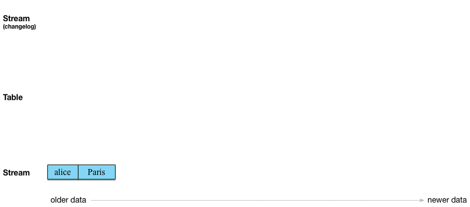
While a table is an aggregation of its input stream, it also has its own output stream! Similar to change data capture (CDC) in databases, every change or mutation of a table in Kafka is captured behind the scenes in an internally used stream of changes aptly called the table’s changelog stream. Many computations in Kafka Streams and KSQL are actually performed on a table’s changelog stream rather than directly on the table. This enables Kafka Streams and KSQL to, for example, correctly re-process historical data according to event-time processing semantics – remember, a stream represents the present and the past, whereas a table can only represent the present (or, more precisely, a snapshot in time).
KTable#toStream().
Here is the first use case example, now with the table’s changelog stream being shown:

Note how the table’s changelog stream is a copy of the table’s input stream. That’s because of the nature of the corresponding aggregation function (UPSERT). And if you’re wondering “Wait, isn’t this 1:1 copying a waste of storage space?” – Kafka Streams and KSQL perform optimizations under the hood to minimize needless data copies and local/network IO. I ignore these optimizations in the diagram above to better illustrate what’s happening in principal.
And, lastly, the second use case example including changelog stream. Here, the table’s changelog stream is different from the table’s input stream because the aggregation function, which performs per-key counting, is different.
But these internal changelog streams also have architectural and operational impacts. Changelog streams are continuously backed up and stored as topics in Kafka, and thereby part of the magic that enables elasticity and fault-tolerance in Kafka Streams and KSQL. That’s because they allow moving processing tasks across machines/VMs/containers without data loss and during live operations, regardless of whether the processing is stateless or stateful. A table is part of your application’s (Kafka Streams) or query’s (KSQL) state, hence it is mandatory for Kafka to ensure that it can move not just the processing code (this is easy) but also the processing state including tables across machines in a fast and reliable manner (this is much harder). Whenever a table needs to be moved from client machine A to B, what happens behind the scenes is that, at the new destination B, the table is reconstructed from its changelog stream in Kafka (server-side) to exactly how it was on machine A. We can see this in the last diagram above, where the “counting table” can be readily restored from its changelog stream without having to reprocess the input stream.
The Stream-Table Duality
The term stream-table duality refers to the above relationship between streams and tables. It means, for example, that you can turn a stream into a table into a stream into a table and so on. See Confluent’s blog post Introducing Kafka Streams: Stream Processing Made Simple for further information.
Turning the Database Inside-Out
In addition to what we covered in the previous sections, you might have come across the article Turning the Database Inside-Out, and now you might be wondering what’s the 10,000 feet view of all this? While I don’t want to go into much detail here, let me briefly juxtapose the world of Kafka and stream processing with the world of databases. Caveat emptor: black-and-white simplifications ahead.
In databases, the first-order construct is the table. This is what you work with. “Streams” also exist in databases, for example in the form of MySQL’s binlog or Oracle’s Redo Log, but they are typically hidden from you in the sense that you do not interact with them directly. A database knows about the present, but it does not know about the past (if you need the past, fetch your backup tapes which, haha, are hardware streams).
In Kafka and stream processing, the first-order construct is the stream. Tables are derivations of streams, as we have seen above. Kafka knows about the present but also about the past. As an example of anecdotal evidence, The New York Times store all articles ever published – 160 years of journalism going back to the 1850’s – in Kafka as the source of truth.
A database thinks table first, stream second. Kafka thinks stream first, table second. In short: A database thinks table first, stream second. Kafka thinks stream first, table second. That said, the Kafka community has realized that most streaming use cases in practice require both streams and tables – even the infamous yet simple WordCount, which aggregates a stream of text lines into a table of word counts, like our second use case example above. Hence Kafka helps you to bridge the worlds of stream processing and databases by providing native support for streams and tables via Kafka Streams and KSQL in order to save you from a lot of DIY pain (and pager alerts). We might call Kafka and the type of streaming platform it represents therefore stream-relational rather than stream-only.
Wrapping Up
I hope you find these explanations useful to better understand streams and tables in Kafka and in stream processing at large. Now that we have finished our closer look, you might want to go back to the beginning of the article to re-read the “Streams and Tables in Plain English” and “Streams and Tables in Kafka English” sections one more time.
If this article made you curious to try out stream-relational processing with Kafka, Kafka Streams, and KSQL, you might want to continue with:
- Learning how to use KSQL, the streaming SQL engine for Kafka, to process your Kafka data without writing any programming code. That’s what I would recommend as your starting point, particularly if you are new to Kafka or stream processing, as you should get up and running in a matter of minutes. There’s also a cool KSQL clickstream demo (including a Docker variant) where you can play with a Kafka, KSQL, Elasticsearch, Grafana setup to drive a real-time dashboard.
- Learning how to build Java or Scala applications for stream processing with the Kafka Streams API.
- And yes, you can of course combine the two, e.g. you can start processing your data with KSQL, then continue with Kafka Streams, and then follow-up again with KSQL.
Regardless of whether you are using Kafka Streams or KSQL, thanks to Kafka you’ll benefit from elastic, scalable, fault-tolerant, distributed stream processing that runs everywhere (containers, VMs, machines, locally, on-prem, cloud, you name it). Just saying in case this isn’t obvious. :-)
Lastly, I titled this article as Part 1 of Streams and Tables. And while I already have ideas for Part 2, I’d appreciate questions or suggestions on what I could cover next. What do you want to learn more about? Let me know in the comments below or drop me an email!